Mouvement parabolique et accélération (version sans fonction)

Télécharger le pdf

Télécharger le notebook, le csv et la vidéo

Lancer le notebook sur binder (lent)

import numpy as np
import matplotlib.pyplot as plt
%matplotlib inline
import csv

with open("parabole2.csv", "r", encoding="utf-8") as f:
    rparabole = csv.reader(f, delimiter=";")
    tableau=[]
    index_row=0
    N=1
    for row in rparabole:
        if index_row < N:
             index_row = index_row+1
        else :
              for i in range (len(row)):
                if len(tableau) <= i:
                    X = []
                    tableau.append(X)
                try:
                    tableau[i].append(float(row[i].replace(",",'.')))
                except ValueError:
                    print('erreur:contenu de cellule non numérique')
                    continue
    print(tableau)
    t=tableau[0]
    x=tableau[1]
    y=tableau[2]

[[0.24, 0.28, 0.32, 0.36, 0.4, 0.44, 0.48, 0.52, 0.56, 0.6, 0.64, 0.68, 0.72, 0.76, 0.8, 0.84, 0.88, 0.92, 0.96, 1.0, 1.04, 1.08, 1.12, 1.16], [-0.223951998822, -0.343580601208, -0.51009038223, -0.707225408616, -0.904090917691, -1.06952262947, -1.26584910392, -1.46177130241, -1.61175563285, -1.78383296605, -1.97894661261, -2.17352122454, -2.35318748976, -2.53150616842, -2.71835708968, -2.8809588697, -3.06740551499, -3.24478088307, -3.42283004442, -3.60792910316, -3.78490019527, -3.97731866872, -4.13111868882, -4.2990185037], [1.76458242983, 1.97872907661, 2.22294809106, 2.45118719902, 2.66398567058, 2.84644213942, 3.02835933818, 3.18711558233, 3.36984168622, 3.49040079194, 3.60283512689, 3.68438818904, 3.79709215904, 3.83259294703, 3.91428082671, 3.93461061335, 3.99313753842, 3.97459609901, 3.9946562506, 3.97597999367, 3.93427759966, 3.8923055706, 3.85100762916, 3.73223687067], [-3.35881386319, -3.83926907511, -4.39437831948, -4.6984222285, -4.61537628747, -4.59800458895, -4.6734998329, -4.39648990626, -4.26517089855, -4.53285206253, -4.72307275216, -4.66513122103, -4.53973738179, -4.51201266471, -4.41596392065, -4.41034897667, -4.48905549951, -4.47657956306, -4.52581793104, -4.52774853362, -4.51639558597, -4.33379221852, -4.15861517319, -4.15321687131], [5.54030774149, 5.7088992284, 5.72816977458, 5.44184327251, 4.98744077131, 4.60697343994, 4.32141849032, 4.12782399047, 3.67426409878, 3.02603583823, 2.55077455354, 2.30508951049, 1.88360398803, 1.52476923155, 1.24757155895, 0.925891633931, 0.51693242311, 0.109564808036, -0.143354032685, -0.647506495101, -0.990538125172, -1.24691830515, -1.81555270826, -2.43219952115]]

vx=[]
for i in range (len(x)-1) :
    vxi=(x[i+1]-x[i])/(t[i+1]-t[i])
    vx.append(vxi)

vy=[]
for i in range (len(y)-1) :
    vyi=(y[i+1]-y[i])/(t[i+1]-t[i])
    vy.append(vyi)

ax=[]
for i in range (len(vx)-1) :
    axi=(vx[i+1]-vx[i])/(t[i+1]-t[i])
    ax.append(axi)

ay=[]
for i in range (len(vy)-1) :
    ayi=(vy[i+1]-vy[i])/(t[i+1]-t[i])
    ay.append(ayi)

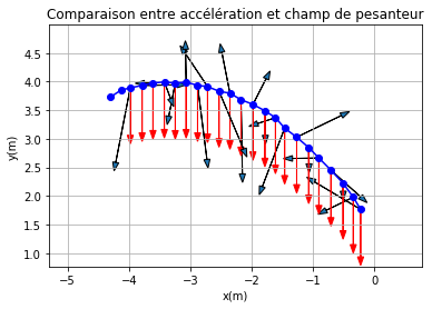
fig = plt.figure()
plt.plot(x,y,'bo-')
for i in range (0, len (ay)):
    plt.arrow(x[i],y[i],0.03*ax[i],0.03*ay[i],head_width=0.1,
              length_includes_head=True)
    plt.arrow(x[i],y[i],0,0.1*(-9.8),fc='r',ec='r',
              head_width=0.1,length_includes_head=True)
plt.xlim(min(x)-1,max(x)+1)
plt.ylim(min(y)-1,max(y)+1)
plt.grid()
plt.xlabel("x(m)")
plt.ylabel("y(m)")
plt.title("Comparaison entre accélération et "
          "champ de pesanteur")
plt.show()

t2=np.array(t[:-2])
axth=0*t2
ayth=0*t2-9.8
coeffax=np.polyfit(t2,ax,0)
axmod=0*t2+coeffax[0]
coeffay=np.polyfit(t2,ay,0)
aymod=0*t2+coeffay[0]
fig = plt.figure()
plt.plot(t2,ay,'bo-',label="ay")
plt.legend()
plt.grid()
plt.ylim(min(ay)-1,max(ay)+1)
plt.plot(t2,ayth,'r-',label="g")
plt.legend()
plt.plot(t2,aymod,'g-',label="moyenne")
plt.legend()
plt.xlabel("temps")
plt.ylabel("accélération verticale")
plt.title("Comparaison entre accélération verticale "
          "et champ de pesanteur vertical")
plt.show()
print("la valeur moyenne de l'accélération verticale est"
      ,round(coeffay[0],1),"m/s²")
plt.plot(t2,ax,'bo-',label="ax")
plt.legend()
plt.grid()
plt.ylim(min(ax)-1,max(ax)+1)
plt.plot(t2,axth,'r-',label="0")
plt.legend()
plt.plot(t2,axmod,'g-',label="moyenne")
plt.legend()
plt.xlabel("temps")
plt.ylabel("accélération horizontale")
plt.title("Comparaison entre accélération horizontale "
          "et champ de pesanteur horizontal")
plt.show()
print("la valeur moyenne de l'accélération horizontale est",
      round(coeffax[0],1),"m/s²")

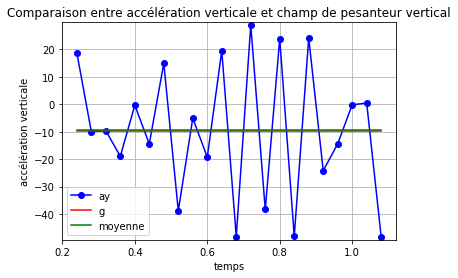
la valeur moyenne de l'accélération verticale est -9.5 m/s²

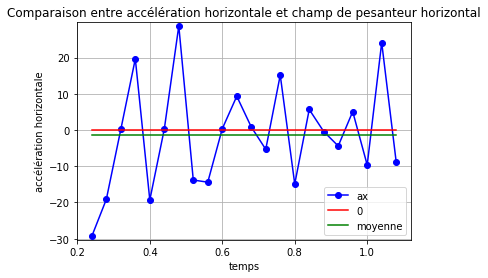
la valeur moyenne de l'accélération horizontale est -1.4 m/s²